
티스토리 뷰
(macOS)[python] curve fitting : (1) regression with scipy/numpy
jinozpersona 2022. 11. 3. 18:14Intro
curve fitting : 커브피팅, 곡선적합, 곡선근사, 곡선피팅, ....
- polynomial regression : 다항식 회귀
- polynomial interpolation : 다항식 보간
curve fitting은 데이터 근사에 사용된다. 오차를 가지는 데이터의 통계적 근사를 regression, 데이터 포인트를 통과하는 곡선을 수치적으로 나타내는 것을 interpolation이라 간단하게 구분할 수 있다. regression, 즉 회귀의 경우는 통계적 추정에 따라 회귀 적합도를 나타내는 R-square(결정계수)이라는 총변동합의 비율로 근사정도를 판단한다.
총 2개의 포스트로 구성되어있다.
(1) polynomial regression : scipy, numpy
(2) polynomial interpolation : scipy
이번 포스트에서는 다항식 회귀(polymonial regression)를 python library scipy와 numpy를 비교해서 다룬다.
Henry's contrant -logK vs. Temp.의 1차/2차/3차 적합을 다룬다.
- scipy.optimize : curve_fit
선형 1차, 2차/3차 함수의 근사 모델을 선언하여 데이터 적합 모델을 찾는 방식
- numpy.polyfit, sklearn.metrices r2_score
numpy의 polyfit 함수(method)에 정의된 다항식 모델로 근사하고 sklearn의 R-square도 구해본다.
Requirements
- Editor : vscode
- python 3.10
- scipy
- numpy
- sklearn
- matplotlib
--용어설명 : curve fitting, regression, interpolation wiki 번역
curve fitting : wiki
....
Curve fitting can involve either interpolation, where an exact fit to the data is required, or smoothing, in which a "smooth" function is constructed that approximately fits the data
한글번역
....
곡선 피팅은 데이터에 대한 정확한 피팅이 요구되는 보간 , 또는 대략적으로 피팅되는 "부드러운" 함수가 생성되는 스무딩 , 중 하나를 포함할 수 있습니다.
polynomial interpolation : wiki
In numerical analysis, polynomial interpolation is the interpolation of a given data set by the polynomial of lowest possible degree that passes through the points of the dataset.
....
Two common explicit formulas for this polynomial are the Lagrange polynomials and Newton polynomials.
한글번역
수치 분석 에서 다항식 보간 은 데이터 세트 의 점을 통과하는 가능한 가장 낮은 차수의 다항식으로 주어진 데이터 세트를 보간 하는 것 입니다.
....
이 다항식에 대한 두 가지 일반적인 명시적 공식은 라그랑주 다항식 과 뉴턴 다항식 입니다.
polynomial regression : wiki
In statistics, polynomial regression is a form of regression analysis in which the relationship between the independent variable x and the dependent variable y is modelled as an nth degree polynomial in x. Polynomial regression fits a nonlinear relationship between the value of x and the corresponding conditional mean of y, denoted E(y |x). Although polynomial regression fits a nonlinear model to the data, as a statistical estimation problem it is linear, in the sense that the regression function E(y | x) is linear in the unknown parameters that are estimated from the data. For this reason, polynomial regression is considered to be a special case of multiple linear regression.
....
Polynomial regression models are usually fit using the method of least squares. The least-squares method minimizes the variance of the unbiased estimators of the coefficients, under the conditions of the Gauss–Markov theorem.
한글번역
통계 에서 다항식 회귀 는 독립 변수 x 와 종속 변수 y 간의 관계를 x 의 n 차 다항식 으로 모델링 하는 회귀 분석 의 한 형태입니다 . 다항식 회귀는 E( y | x )로 표시된 x 값 과 y 의 해당 조건부 평균 사이의 비선형 관계에 맞습니다 . 다항식 회귀 는 비선형 모델을 데이터에 적합 하지만 통계적 추정 으로 회귀 함수 E( y | x )가 데이터 에서 추정된 미지의 매개변수 에서 선형이라는 점에서 문제는 선형 입니다. 이러한 이유로 다항식 회귀는 다중 선형 회귀 의 특수한 경우로 간주됩니다 .
....
다항식 회귀 모델은 일반적으로 최소 자승법 을 사용하여 적합합니다 . 최소제곱법 은 가우스-마르코프 정리 의 조건에서 계수 의 편향되지 않은 추정량 의 분산 을 최소화합니다 . 최소제곱법은 1805년 Legendre 와 Gauss 가 1809년에 발표했습니다 .
1. 이산화탄소(CO2, Carbon Dioxide) 해리상수 pKa1, pKa2
해리될 수 있는 양성자를 2개 이상 포함하는 산을 다양성자산이라하는데 CO2가 대표적이며 물에 용해되어 약산이 되며 2번의 해리 상수(dissociation constants)를 나타낸 표이다.
데이터출처 : chegg.com
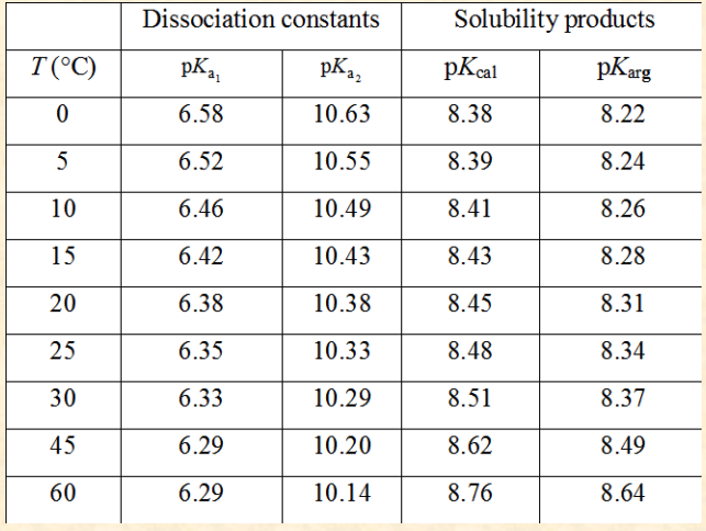
curve fitting 중 regression에 필요한 독립변수를 T(oC)로 두고 pKa1, pKa2를 종속변수로 두었다.
pka1 = -log10[Ka1]과 같으며, python code에서는 T와 K1, K2로 두고 분석하였다.
## data폴더를 하위 폴더로 하여 저장
./data/solubility_data.xlsx
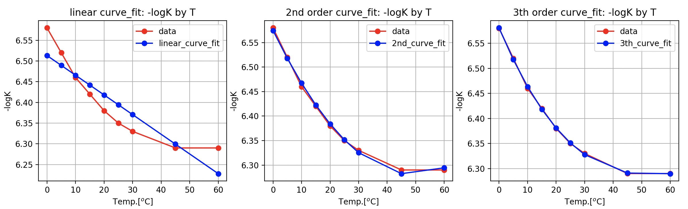
2. polynomial regression : scipy
curvefit_regression_with_scipy.py
import os
from openpyxl import load_workbook as loadwb
import matplotlib.pyplot as plt
import numpy as np
from scipy.optimize import curve_fit as cf


# data path, name, sheet name
fpath = './data/'
fname = 'solubility_data.xlsx'
sh_names = ('pK_CO2','pKH_CO2')

# read excel file
wb = loadwb(os.path.join(fpath,fname), data_only=True)
ws = wb[sh_names[0]]
wb.close()

# cell location
T_rng = ws['A3':'A11']
pK1_rng = ws['B3':'B11']
pK2_rng = ws['C3':'C11']

## convert cell(tuple) to value
def cell2value(rng):
    v = []
    for rng_tuple in rng:
        for cell in rng_tuple:
            v.append(cell.value)
    return v
T = cell2value(T_rng)
pK1 = cell2value(pK1_rng)
pK2 = cell2value(pK2_rng)

# # convert numpy data
T = np.array(T)
K = np.array(pK1)


# estimate model
# herein, linear: 1st order
def fun1(x,a,b):
    return a*x + b
# herein, non-linear: 2nd order
def fun2(x,a,b,c):
    return a*(x**2) + b*x + c
# herein, non-linear: 3th order
def fun3(x,a,b,c,d):
    return a*(x**3) + b*(x**2) +c*x + d

# curve_fit
popt_fun1, pcov_fun1 = cf(fun1,T,K,method="lm")
print("1st order curve_fit [a b] is {}".format(popt_fun1))

popt_fun2, pcov_fun2 = cf(fun2,T,K,method="lm")
print("2nd order curve_fit [a b c] is {}".format(popt_fun2))

popt_fun3, pcov_fun3 = cf(fun3,T,K,method="lm")
print("3th order curve_fit [a b c d] is {}".format(popt_fun3))


# define figure
fig = plt.figure(figsize=(18,8))

# subplot (1,1)
ax1 = fig.add_subplot(2,3,1)
plt.plot(T,K,'ro-',label='data')
plt.plot(T,fun1(T,*popt_fun1),'bo-',label='linear_curve_fit')
plt.title("linear curve_fit: -logK by T")
plt.xlabel("Temp.[$^o$C]")
plt.ylabel("-logK")
plt.grid()
plt.legend()

# subplot (1,2)
ax2 = fig.add_subplot(2,3,2)
plt.plot(T,K,'ro-',label='data')
plt.plot(T,fun2(T,*popt_fun2),'bo-',label='2nd_curve_fit')
plt.title("2nd order curve_fit: -logK by T")
plt.xlabel("Temp.[$^o$C]")
plt.ylabel("-logK")
plt.grid()
plt.legend()

# subplot (1,3)
ax3 = fig.add_subplot(2,3,3)
plt.plot(T,K,'ro-',label='data')
plt.plot(T,fun3(T,*popt_fun3),'bo-',label='3th_curve_fit')
plt.title("3th order curve_fit: -logK by T")
plt.xlabel("Temp.[$^o$C]")
plt.ylabel("-logK")
plt.grid()
plt.legend()

plt.show()
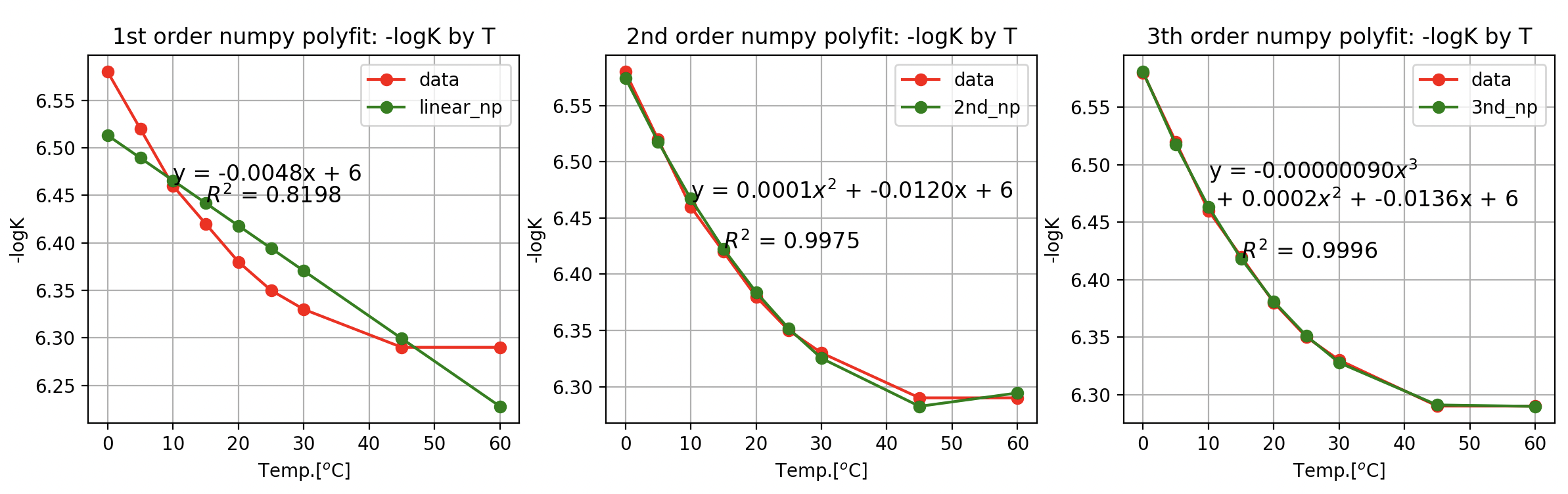
3. polynomial regression : numpy, sklearn
같은 파일에 내용 업데이트
curvefit_regression_with_numpy.py
import os
from openpyxl import load_workbook as loadwb
import matplotlib.pyplot as plt
import numpy as np
from sklearn.metrics import r2_score


# data path, name, sheet name
fpath = './data/'
fname = 'solubility_data.xlsx'
sh_names = ('pK_CO2','pKH_CO2')

# read excel file
wb = loadwb(os.path.join(fpath,fname), data_only=True)
ws = wb[sh_names[0]]
wb.close()

# cell location
T_rng = ws['A3':'A11']
pK1_rng = ws['B3':'B11']
pK2_rng = ws['C3':'C11']

## convert cell(tuple) to value
def cell2value(rng):
    v = []
    for rng_tuple in rng:
        for cell in rng_tuple:
            v.append(cell.value)
    return v
T = cell2value(T_rng)
pK1 = cell2value(pK1_rng)
pK2 = cell2value(pK2_rng)

# # convert numpy data
T = np.array(T)
K = np.array(pK1)
# K = np.array(pK2)

#### numpy polyfit
polyfit_1 = np.polyfit(T,K,1)
polyfit_2 = np.polyfit(T,K,2)
polyfit_3 = np.polyfit(T,K,3)

print(K)
print("1st order polyfit [a b] is {}".format(polyfit_1))
print("2nd order polyfit [a b c] is {}".format(polyfit_2))
print("3th order polyfit [a b c d] is {}".format(polyfit_3))

# estimated K by polyfit
est_K_fit_1 = polyfit_1[0]*T + polyfit_1[1]
est_K_fit_2 = polyfit_2[0]*(T**2) + polyfit_2[1]*T + polyfit_2[2]
est_K_fit_3 = polyfit_3[0]*(T**3) + polyfit_3[1]*(T**2) + polyfit_3[2]*T + polyfit_3[3]

#### numpy polyfit : R2(R-square)
R2_fit_1 = r2_score(K,est_K_fit_1)
R2_fit_2 = r2_score(K,est_K_fit_2)
R2_fit_3 = r2_score(K,est_K_fit_3)

print(R2_fit_1)
print(R2_fit_2)
print(R2_fit_3)


fig2 = plt.figure(figsize=(18,8))
# subplot (1,1)
ax1 = fig2.add_subplot(2,3,1)
plt.plot(T,K,'ro-',label='data')
plt.plot(T,est_K_fit_1,'go-',label='linear_np')
plt.title("1st order numpy polyfit: -logK by T")
plt.xlabel("Temp.[$^o$C]")
plt.ylabel("-logK")
plt.grid()
plt.legend()
plt.text(T[2], est_K_fit_1[2], 'y = %.4fx + %d'%(polyfit_1[0],polyfit_1[1]), size = 12)
plt.text(T[3], est_K_fit_1[3], '$R^2$ = %.4f'%R2_fit_1, size = 12)

# subplot (1,2)
ax2 = fig2.add_subplot(2,3,2)
plt.plot(T,K,'ro-',label='data')
plt.plot(T,est_K_fit_2,'go-',label='2nd_np')
plt.title("2nd order numpy polyfit: -logK by T")
plt.xlabel("Temp.[$^o$C]")
plt.ylabel("-logK")
plt.grid()
plt.legend()
plt.text(T[2], est_K_fit_2[2], 'y = %.4f$x^2$ + %.4fx + %d'%(polyfit_2[0], polyfit_2[1], polyfit_2[2]), size = 12)
plt.text(T[3], est_K_fit_2[3], '$R^2$ = %.4f'%R2_fit_2, size = 12)

# subplot (1,3)
ax3 = fig2.add_subplot(2,3,3)
plt.plot(T,K,'ro-',label='data')
plt.plot(T,est_K_fit_3,'go-',label='3nd_np')
plt.title("3th order numpy polyfit: -logK by T")
plt.xlabel("Temp.[$^o$C]")
plt.ylabel("-logK")
plt.grid()
plt.legend()
plt.text(T[2], est_K_fit_3[2], 'y = %.8f$x^3$\n + %.4f$x^2$ + %.4fx + %d'%(polyfit_3[0],polyfit_3[1], polyfit_3[2], polyfit_3[3]), size = 12)
plt.text(T[3], est_K_fit_3[3], '$R^2$ = %.4f'%R2_fit_3, size = 12)

plt.show()# # convert numpy data
T = np.array(T)
K = np.array(pK1)
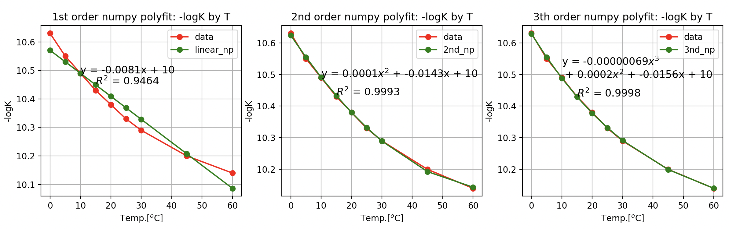
K == pK2 일때
# # convert numpy data
T = np.array(T)
K = np.array(pK2)
K1에서 R2 = 99.96%
K2에서 R2 = 99.98%
0~60도 온도 구간에서는 3차 다항식 적합한 곡선이 근사값에 가깝다고 해석할 수 있다.
curve_fit / polyfit 모두 3차 다항식 회귀에 가장 적합.
'python > Data Science' 카테고리의 다른 글
| (macOS)[python] curve fitting : (2) interpolation with scipy (0) | 2022.11.04 |
|---|---|
| (macOS)[python] 공공데이터포탈 data.go.kr OpenAPI 활용 (0) | 2022.10.13 |
| (macOS)[python] 파일이름 encoding, 한글 자모분리 해결 (0) | 2022.02.27 |
| (macOS)[python] 기상청 RSS 서비스를 이용한 데이터 parsing (0) | 2021.02.15 |
| (macOS)[python] IP address 확인 : Public/Pravate(Virtual) (0) | 2021.02.15 |
- Total
- Today
- Yesterday
- Django
- sublime text
- DAQ
- template
- 코로나
- Pandas
- COVID-19
- CSV
- 코로나19
- pyserial
- Python
- Raspberry Pi
- vscode
- Model
- arduino
- Templates
- MacOS
- 라즈베리파이
- ERP
- Regression
- SSH
- 확진
- 자가격리
- server
- DS18B20
- r
- github
- raspberrypi
- git
- analysis
| 일 | 월 | 화 | 수 | 목 | 금 | 토 |
|---|---|---|---|---|---|---|
| 1 | 2 | 3 | ||||
| 4 | 5 | 6 | 7 | 8 | 9 | 10 |
| 11 | 12 | 13 | 14 | 15 | 16 | 17 |
| 18 | 19 | 20 | 21 | 22 | 23 | 24 |
| 25 | 26 | 27 | 28 | 29 | 30 | 31 |